
elevne's Study Note
딥러닝 파이토치 교과서 (4: 합성곱신경망 (2)) 본문
이번에는 예제 코드, 데이터를 활용하여 CNN 을 직접 코드로 구현해보았다. 우선 필요한 라이브러리들을 import 하고, 가능하다면 device 를 GPU 로 설정해준다.
import numpy as np
import matplotlib.pyplot as plt

import torch
import torch.nn as nn
from torch.autograd import Variable
import torch.nn.functional as F

import torchvision
import torchvision.transforms as transforms
from torch.utils.data import Dataset, DataLoader

device = torch.device("cuda:0" if torch.cuda.is_available() else "cpu")
print(device)

이번 실습에서 사용된 Fashion MNIST 데이터는 torchvision 을 통해서 다운로드 받을 수 있다. 다운로드 시 첫 번째 파라미터로 다운로드 경로를 설정해줄 수 있으며, 두 번째 인자(download)를 True 로 설정하면 첫 번째 인자의 위치에 해당 데이터셋이 있는지 확인한 후 다운로드를 진행한다. 또 tranform 인자를 받는데, 이는 이미지를 텐서로 변환해주는 역할을 한다.
train_dataset = torchvision.datasets.FashionMNIST("/content/drive/MyDrive/Colab Notebooks/딥러닝파이토치/data", download=True, transform=transforms.Compose([transforms.ToTensor()]))
test_dataset = torchvision.datasets.FashionMNIST("/content/drive/MyDrive/Colab Notebooks/딥러닝파이토치/data", download=True, train=False, transform=transforms.Compose([transforms.ToTensor()]))
다운로드 받은 Fashion MNIST 데이터는 DataLoader 객체 안에 담아서 메모리로 불러올 수 있다. DataLoader() 을 사용하면 원하는 크기의 배치 단위로 데이터를 불러올 수 있다. shuffle = True 로 설정하면 순서가 무작위로 섞이게도 할 수 있다.
train_loader = DataLoader(train_dataset, batch_size=100)
test_loader = DataLoader(test_dataset, batch_size=100)
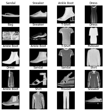
모델을 정의해주기 전에 우선 데이터를 임의로 추출하여 시각화해보았다. 아래와 같은 코드로 진행하였다.
labels_map = {
    0 : "T-Shirt",
    1 : "Trouser",
    2 : "Pullover",
    3 : "Dress",
    4 : "Coat",
    5 : "Sandal",
    6 : "Shirt",
    7 : "Sneaker",
    8 : "Bag",
    9 : "Ankle Boot"
}

fig = plt.figure(figsize=(8, 8))
columns = 4
rows = 5
for i in range(1, columns * rows + 1):
  img_xy = np.random.randint(len(train_dataset))
  img = train_dataset[img_xy][0][0, :, :]
  fig.add_subplot(rows, columns, i)
  plt.title(labels_map[train_dataset[img_xy][1]])
  plt.axis("off")
  plt.imshow(img, cmap="gray")
plt.show()
DNN 과 CNN 의 성능을 비교해보기 위해 우선 DNN Model 을 정의하고 훈련을 시켜보았다. DNN 코드는 아래와 같다.
class FashionDNN(nn.Module):
  def __init__(self):
    super(FashionDNN, self).__init__()
    self.fc1 = nn.Linear(in_features = 784, out_features = 256)
    self.drop = nn.Dropout(0.25)
    self.fc2 = nn.Linear(in_features = 256, out_features = 128)
    self.fc3 = nn.Linear(in_features = 128, out_features = 10)
  def forward(self, input_data):
    out = input_data.view(-1, 784)
    out = F.relu(self.fc1(out))
    out = self.drop(out)
    out = F.relu(self.fc2(out))
    out = self.fc3(out)
    return out
torch 에서 모델 클래스를 작성할 때는 항상 torch.nn.Module 을 상속받도록 한다. nn 은 딥러닝 모델 (네트워크) 구성에 필요한 모듈이 모여있는 패키지이며, Linear() 은 단순한 선형회귀 모델을 만들 때 사용된다. in_features 와 out_features 를 파라미터로 받게된다. forward() 함수 내에서 사용된 view 메서드는 넘파이의 reshape 메서드와 같은 역할로, 텐서의 크기를 변경해주는 역할을 한다.
learning_rate = 0.001
model = FashionDNN()
model.to(device)
criterion = nn.CrossEntropyLoss()
optimizer = torch.optim.Adam(model.parameters(), lr=learning_rate)

num_epochs = 5
count = 0
loss_list = []
iteration_list = []
accuracy_list = []
predictions_list = []
labels_list = []

for epoch in range(num_epochs):
  for images, labels in train_loader:
    images, labels = images.to(device), labels.to(device)
    train = Variable(images.view(100, 1, 28, 28))
    labels = Variable(labels)
    outputs = model(train)
    loss = criterion(outputs, labels)
    optimizer.zero_grad()
    loss.backward()
    optimizer.step()
    count += 1
    if not (count % 50):
      total = 0
      correct = 0
      for images, labels in test_loader:
        images, labels = images.to(device), labels.to(device)
        labels_list.append(labels)
        test = Variable(images.view(100, 1, 28, 28))
        outputs = model(test)
        predictions = torch.max(outputs, 1)[1].to(device)
        predictions_list.append(predictions)
        correct += (predictions == labels).sum()
        total += len(labels)
      accuracy = correct * 100 / total
      loss_list.append(loss.data)
      iteration_list.append(count)
      accuracy_list.append(accuracy)
    if not (count % 500):
      print("Iteration: {}, Loss: {}, Accuracy: {}".format(count, loss.data, accuracy))
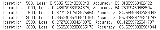
모델의 optimizer 은 Adam, loss function 은 Cross Entropy 가 사용되었다. 학습을 진행할 때 images.to(device), labels.to(device) 와 같이 작성하였는데 이는 모델이 데이터를 처리하기 위해서는 모델과 데이터가 동일한 장치에 있어야하기 때문이다. 그 후에 데이터를 autograd 에서 import 한 Variable 객체 안에 넣어준다. 이는 torch 에서 자동 미분을 수행하는 핵심 패키지로, 자동 미분에 대한 값을 저장하기 위해 tape 를 사용한다. 순전파 단계에서 tape 는 수행하는 모든 연산을 저장한다. 그리고 역전파 단계에서 저장된 값들을 꺼내서 사용하는 것이다. Autograd 는 Variable 을 사용해서 역전파를 위한 미분 값을 자동으로 계산해주는 것이다. 5 번의 epoch 을 거치면서 약 87 % 의 Accuracy 가 나온 것을 확인할 수 있었다. 그 다음에는 CNN 모델을 정의해주었다.
class FashionCNN(nn.Module):
  def __init__(self):
    super(FashionCNN, self).__init__()
    self.layer1 = nn.Sequential(
        nn.Conv2d(in_channels=1, out_channels=32, kernel_size=3, padding=1),
        nn.BatchNorm2d(32),
        nn.ReLU(),
        nn.MaxPool2d(kernel_size=2, stride=2)
    )
    self.layer2 = nn.Sequential(
        nn.Conv2d(in_channels=32, out_channels=64, kernel_size=3),
        nn.BatchNorm2d(64),
        nn.ReLU(),
        nn.MaxPool2d(2)
    )
    self.fc1 = nn.Linear(in_features=64*6*6, out_features=600)
    self.drop = nn.Dropout(0.25)
    self.fc2 = nn.Linear(in_features=600, out_features=120)
    self.fc3 = nn.Linear(in_features=120, out_features=10)
  def forward(self, x):
    out = self.layer1(x)
    out = self.layer2(out)
    out = out.view(out.size(0), -1)
    out = self.fc1(out)
    out = self.drop(out)
    out = self.fc2(out)
    out = self.fc3(out)
    return out
위에서는 DNN 과 다르게 nn.Sequential 을 사용하였다. 이를 사용하면 __init__() 에서 사용할 네트워크 모델을 정의해줄 뿐만 아니라 forward 함수에서 구현될 순전파를 계층 형태로 좀 더 가독성이 뛰어난 코드로 작성할 수 있다고 한다. nn.Sequentail 내에서 nn.Conv2d 를 사용하여 합성곱 연산을 통해 이미지의 특징을 추출한다. 파라미터로 in_channels (입력 채널의 수, Gray Scale 이면 1, RGB 이면 3 을 가지는 경우가 많다) , out_channels (출력 채널의 수) , kernel_size (커널 크기), padding (패딩 크기, 입력 데이터 주위에 0 을 채우는 것) 을 받는다. 그 후 BatchNorm2d 로 각 배치 단위별로 데이터가 다양한 분포를 가지더라도 평균과 분산을 이용하여 정규화해준다. 분포를 가우시안 형태로 만들 수 있는 것이다. 다음은 MaxPool2d 를 사용하여 이미지 크기를 축소시킨다. kernel 과 stride 를 인자로 받는다. Conv2d layer 을 쌓은 출력크기를 계산해주고 Fully Connected Layer 로 이어주어야 하는데, 이는 다음 시간에 알아볼 예정이다. 작성한 CNN 모델 또한 위에서 사용한 학습 코드와 동일한 코드를 사용하여 학습시킨다. 결과는 아래와 같다.
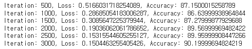
DNN 보다 결과가 발전된 것을 확인할 수 있다.
Reference:
딥러닝 파이토치 교과서

'Machine Learning > Pytorch' 카테고리의 다른 글
| 딥러닝 파이토치 교과서 (4-2: CNN 전이학습) (0) | 2023.03.11 |
|---|---|
| 딥러닝 파이토치 교과서 (4-1: CNN Conv2d, MaxPool2d 계산) (0) | 2023.03.06 |
| 딥러닝 파이토치 교과서 (4: 합성곱신경망 (1)) (0) | 2023.03.04 |
| 딥러닝 파이토치 교과서 (3: 딥러닝 기초 정리) (0) | 2023.03.03 |
| 딥러닝 파이토치 교과서 (2-2: 비지도학습(2)) (0) | 2023.03.02 |


